Diagnostic plots for a segmentation

Four views of a segment_survey() result, each answering a question that is hard to answer from the tables. Returns a ggplot object, so it can be modified, saved, or faceted further like any other.

Usage

# S3 method for class 'distsamp_segments'
plot(
  x,
  what = c("segments", "tracks", "effort", "distances"),
  species = NULL,
  coastline = FALSE,
  max_legend = 8,
  dates = NULL,
  years = NULL,
  months = NULL,
  sightings = TRUE,
  ...
)

Arguments

x: A distsamp_segments object from segment_survey().
what: Which view: "segments" (default), "tracks", "effort", or "distances".
species: Optional character vector of SPECCODE values to show, for the views that draw sightings. NULL (default) shows all.
coastline: Land to draw under the map views. FALSE (default) draws none. TRUE fetches Natural Earth countries through rnaturalearth; a scale name — "small", "medium", "large" — picks the resolution; or pass your own sf object. Ignored by the "effort" and "distances" views. See the note on resolution below.
max_legend: Most groups to name in the legend. Default 8. Species beyond it are gathered into one "other" entry — they stay on the map, they just stop having their own colour — and tracks beyond it take a recycled palette with the legend dropped. A survey with 36 species or 130 tracks produces a legend that squeezes the map to nothing otherwise.
dates, years, months: Which survey days to draw, passed to filter_days(). NULL (default) draws all of them. Every table in the object — points, segments, detections — is cut to the same days.
sightings: Draw the sightings over the segments? Default TRUE. Set FALSE on the whole-archive segments view: 2,204 markers over 8,628 segments cover the colouring that says where the cuts fall, which is what that view is for. The per-day figures are where a sighting's position against its segment can actually be read.
...: Ignored, for compatibility with plot().

Value

A ggplot object.

What each view is for

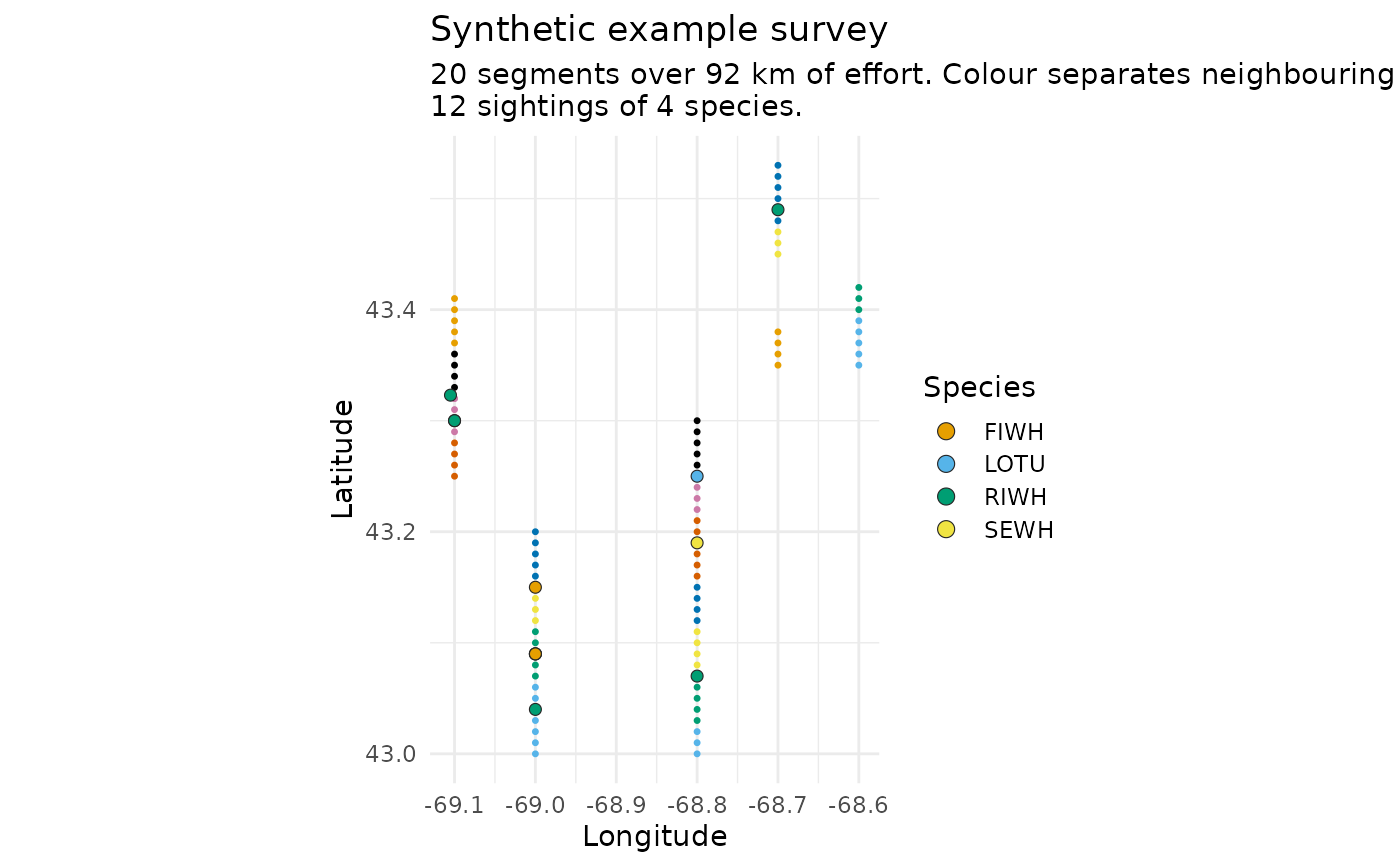
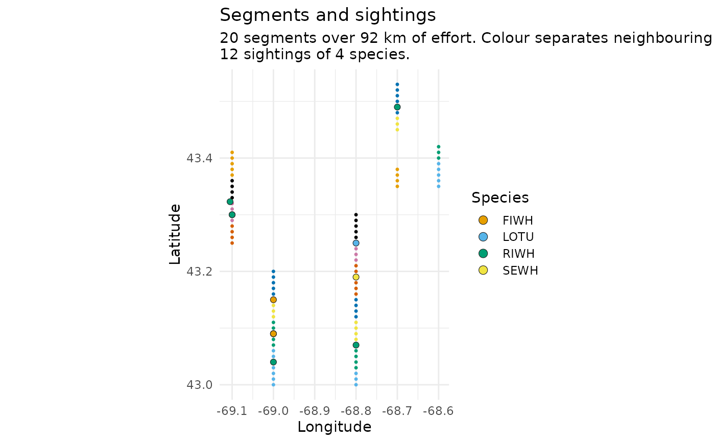
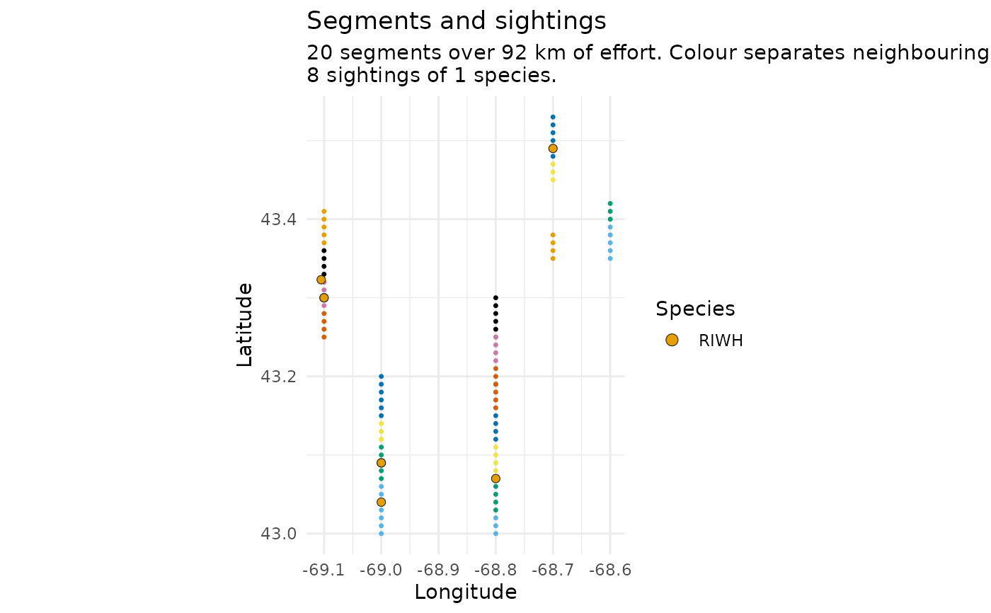
"segments": The track flown, the segment midpoints, and where the sightings were. The first thing to look at: a segmentation that has gone wrong is usually obvious here, as midpoints strung along a line the aircraft never flew, or clustered where a track should have been split.
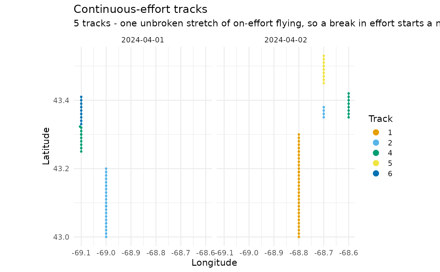
"tracks": The same positions coloured by new_trackno, faceted by date. This is the view that shows whether split_tracks() did the right thing — a break in effort should start a new colour, and a colour should never span two places the aircraft could not have flown between.
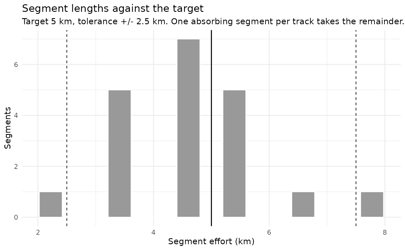
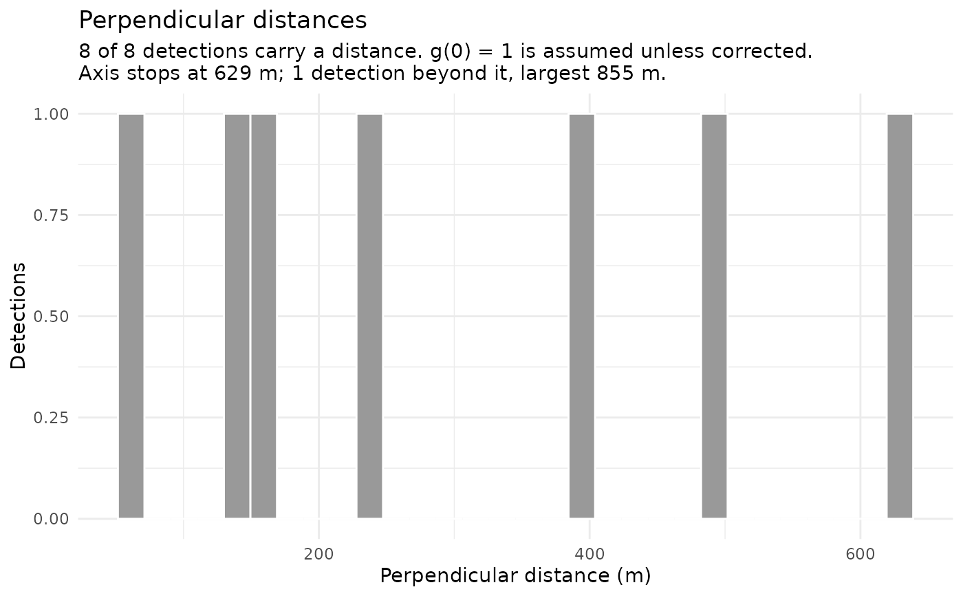
"effort": Segment lengths against the target. The Becker method produces segments near seg_length but not at it, with one absorbing segment per track taking up the remainder, so a spread is expected. What is not expected is mass outside the tolerance band, which the dashed lines mark.
"distances": The distribution of perpendicular distances. This is the detection-function diagnostic: look for a shoulder near zero and a tail that falls away. A spike at zero, a peak away from zero, or a long flat tail all mean something, and all of them matter before Distance::ds() is called. See the note on g(0) below. The axis stops at the 99th percentile and the subtitle reports what lies beyond it: a single implausible distance would otherwise set the scale and put every real one in the first bin. Since such a distance is a bug worth finding rather than a nuisance worth hiding, the subtitle says outright when the largest is too far to be a detection.

Coastlines, and why the default is none

coastline = TRUE draws Natural Earth land under the track. That is enough to orient a shelf-scale survey, and not enough for a bay. Natural Earth's medium scale is 1:50,000,000; against a survey whose lines are a few kilometres apart, its shoreline is wrong by more than the thing you are looking at, and a segmentation that hugs the coast will appear to run over land.

So: use it to get your bearings, and pass your own sf object for anything anyone else will see.

plot(segs, coastline = sf::st_read("gshhg_cape_cod.shp"))

scale = "large" (1:10m) is better and needs rnaturalearthhires, which is not on CRAN — install it from the rOpenSci r-universe.

On reading the distance histogram

A dip in the first bin is not necessarily a sampling artefact — an aircraft cannot see the water directly beneath it, and for the Skymaster the handbook says so explicitly (8.A.31). That is a reason to truncate on the left, not to assume the animals were not there. Neither is a smooth curve evidence that g(0) = 1: animals submerged when the aircraft passed leave no trace in this plot at all. See docs/07-fitting-architecture.md in the package repository.

Examples

path <- system.file("extdata", "narwc-example.csv", package = "distsamp")
segs <- segment_survey(read_narwc(path), seg_length = 5, seed = 1)
#> `read_narwc()` renamed 2 columns:
#>   LAT_DD  -> LATITUDE
#>   LONG_DD -> LONGITUDE
#> All matched an exact entry in the alias table; `narwc_column_mapping()` returns this, and `quiet = TRUE` silences it.

# Where the segments are, and what was seen
plot(segs)


# Did track splitting do the right thing? A break in effort should start a
# new colour.
plot(segs, what = "tracks")


# Are segment lengths near the target? Dashed lines are the tolerance band.
plot(segs, what = "effort")


# The detection-function diagnostic, before handing anything to Distance
plot(segs, what = "distances")


# Just one species
plot(segs, species = "RIWH")


# It is an ordinary ggplot, so keep going
plot(segs) + ggplot2::labs(title = "Synthetic example survey")