Look at the survey partway through the pipeline

Draws the records as they stand at whatever stage they have reached, so a segmentation can be checked before it is trusted. plot() on a distsamp_segments object shows the finished result; this shows the steps that produced it, where a mistake is still legible.

Usage

plot_survey(
  dat,
  what = c("effort", "occupations", "tracks", "platform", "legstage", "raw", "positions"),
  coastline = TRUE,
  max_points = 50000,
  max_legend = 12,
  facet_by = NULL,
  dates = NULL,
  years = NULL,
  months = NULL,
  sightings = FALSE
)

Arguments

dat: A survey data frame at any stage: LATITUDE and LONGITUDE are required, and each view needs the column it colours by.
what: Which view: "effort" (default), "occupations", "tracks", "platform", "legstage", "raw", or "positions".
coastline: Land to draw underneath. TRUE (default) fetches Natural Earth through rnaturalearth; FALSE draws none; a scale name — "small", "medium", "large" — picks the resolution; or pass your own sf, which is the better option at bay scale. Unlike plot.distsamp_segments(), a coastline that cannot be fetched here warns and draws nothing rather than erroring: this is a look-at-it function, and losing the land is better than losing the plot.
max_points: Thin to at most this many records. Default 50000.
max_legend: Most groups to name in the legend. Default 12. Beyond this, occupations and tracks take a recycled palette and the legend is dropped — a hundred labels is not a legend, and a hundred colours cannot be told apart.
facet_by: Column to facet on, or NULL for none. Defaults to DATE when the data covers 2 to 12 days — beyond that the panels are too small to read, and one map of everything is more use.
dates, years, months: Which survey days to draw, passed to filter_days(). NULL (default) draws all of them. A decade of survey on one map is a smear; years = 2019, months = 8 is a question a map can answer.
sightings: Draw the sightings over the effort? FALSE (default) draws none, TRUE draws every species, and a character vector of SPECCODE values draws only those — sightings = "RIWH". They are taken from the data before thinning, since a few thousand sighting rows in three million would not survive it, and are drawn as outlined markers so they read on top of the track rather than as more of it.

Value

A ggplot object.

What each view is for

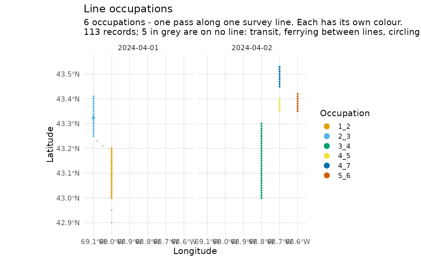
"effort": Positions coloured by OnOff.Effort. The first thing to look at: a survey that is almost entirely off effort has a criterion failing, and the map says whether it is everywhere or on particular days.
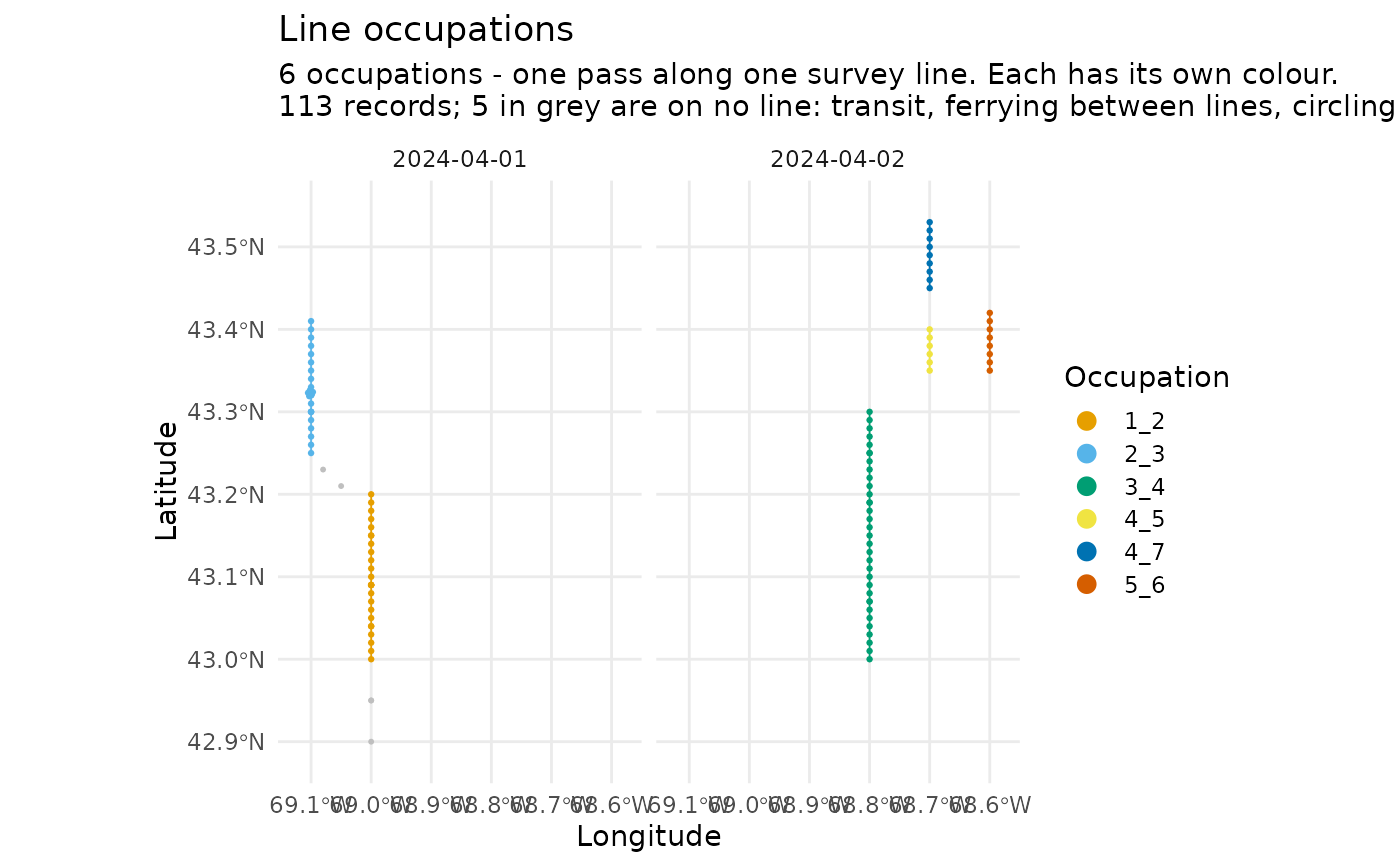
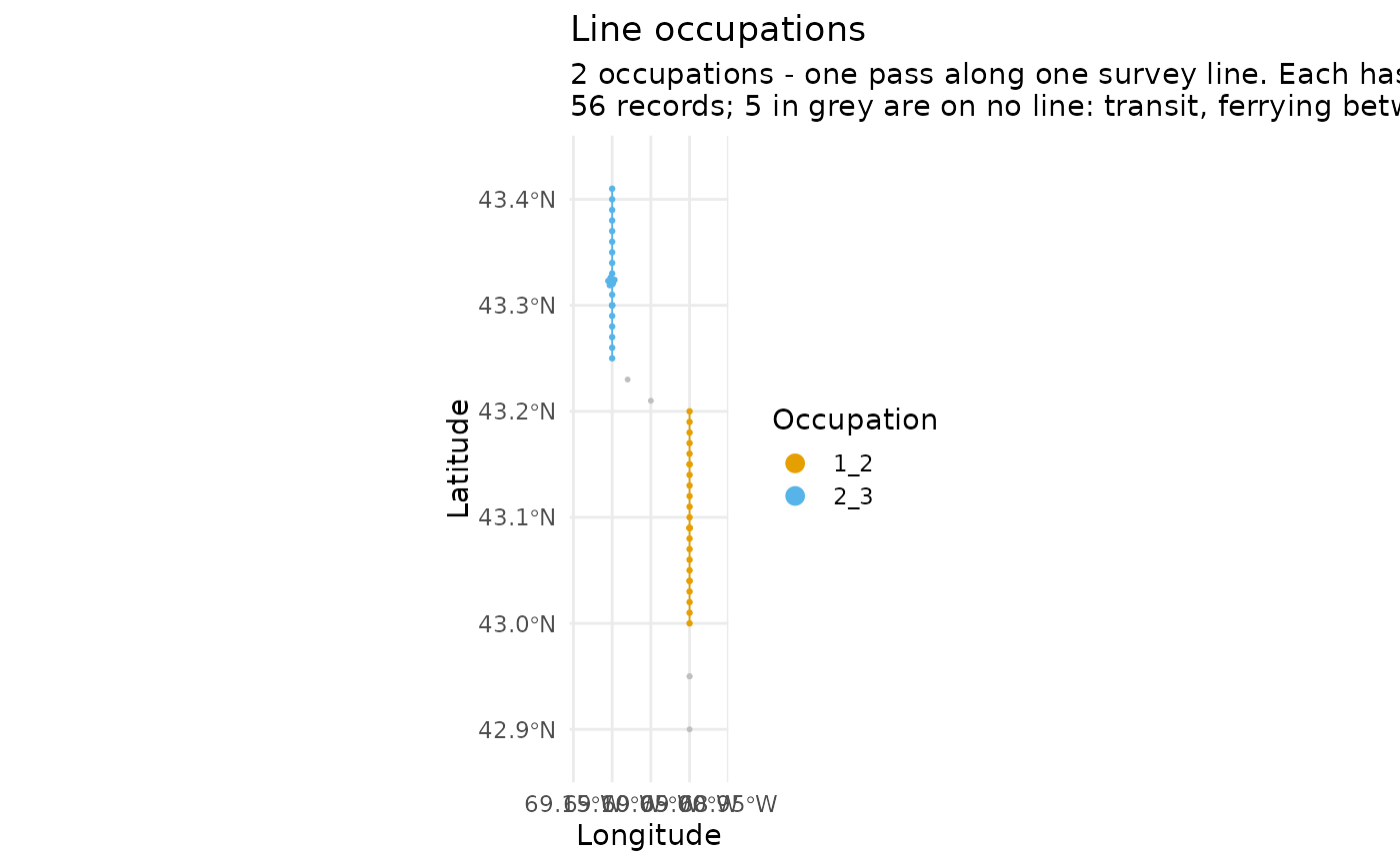
"occupations": Positions coloured by LEGNO3, the line-occupation identifier. Adjacent occupations take different colours, so a line that should be one occupation and is drawn in three — or three that are drawn as one — is visible immediately. This is the view that catches a bad make_leg_id(), and a bad LEGNO3 is the single most consequential thing that can go wrong: effort is grouped by it and segments are cut within it.
"tracks": Positions coloured by new_trackno, the stretches of continuous effort that are actually chopped into segments. Differs from "occupations" wherever effort broke mid-line.
"platform": Positions coloured by PLATFORM_KIND from narwcr::classify_platform(). For an archive holding more than one kind of survey.
"legstage": Positions coloured by LEGSTAGE. Shows where a line begins, breaks off, resumes and ends — and, on a file that records the code only at change points, how little of it is written down.
"raw": Every position, coloured by LEGTYPE, needing nothing but the file as read. What the survey looks like before any of this package has touched it — the view to compare the others against when a later stage seems to have lost something.
"positions": Every position, uncoloured. The only view that cannot fail for want of a column: it needs LATITUDE and LONGITUDE and nothing else, so it works on a file that has not been through prepare_aerial(), or one whose columns are not what you expected. Where "raw" still asks for LEGTYPE, this asks for nothing. Add sightings = TRUE and it is the whole survey — effort and what was seen on it — in one map.

Thinning

A survey archive can hold millions of positions, and a scatter plot of five million points is neither drawable nor readable. The plotted points are thinned to max_points by taking every nth. The subtitle says when it happened. Set max_points = Inf to draw every point.

Thinning never applies to the path. Every nth preserves the shape of a straight line and loses it at every turn, so a path drawn through the survivors cuts the corners: at three million records that is a chord between fixes some 18 km apart, and against a coastline it draws a trackline over land that is not in the data. The lines in the "occupations" and "tracks" views are therefore built from every fix, whatever max_points says. On a whole archive that costs a few seconds of drawing, and it buys a map that does not invent a mistake for you to go looking for.

Examples

path <- system.file("extdata", "narwc-example.csv", package = "distsamp")
dat <- narwcr::flag_effort(narwcr::make_leg_id(narwcr::read_narwc(path, quiet = TRUE)))
plot_survey(dat, "occupations")


# One day, or one month of one year
plot_survey(dat, "occupations", dates = "2024-04-01")

plot_survey(dat, "occupations", years = 2024, months = "April")