Map where a projection leaves the conditions the model was fitted under

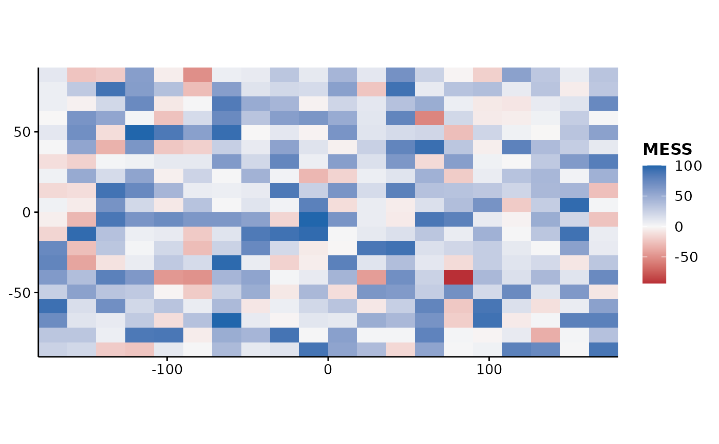
Draws a MESS surface: cells below zero are outside the training range of at least one covariate, and predictions there are extrapolations.

Usage

plotExtrapolation(
  x,
  training = NULL,
  vars = NULL,
  title = "",
  legend.lab = "MESS",
  novel.only = FALSE,
  max.cells = 5e+05,
  theme = theme_fancyfx()
)

Arguments

x: A SpatRaster of covariates, or a single-layer raster already holding MESS values.
training: A data frame of training covariate values, or a fitted model to take them from. Required unless x is already a MESS surface.
vars: Covariates to consider.
title: Plot title, optional.
legend.lab: Legend title.
novel.only: Whether to show only the novel cells, hiding everything within the training range.
max.cells: Largest number of cells to draw; above this the raster is aggregated and the plot says so.
theme: A ggplot2 theme. Defaults to theme_fancyfx().

Value

A ggplot2 object.

Details

The scale is diverging about zero, because zero is a real boundary and not a midpoint of convenience: on one side the model is interpolating, on the other it is guessing. A sequential scale would hide that edge in a smooth ramp. The two poles are red and blue rather than red and green, so the distinction survives the most common colour vision deficiencies.

See mess() for what this does and does not detect – in particular, it cannot see novel combinations of individually ordinary covariates.

References

Elith, J., Kearney, M., & Phillips, S. (2010). The art of modelling range-shifting species. Methods in Ecology and Evolution, 1(4), 330-342. doi:10.1111/j.2041-210X.2010.00036.x

Examples

if (requireNamespace("terra", quietly = TRUE)) {
  set.seed(1)
  training <- data.frame(temp = rnorm(200, 10, 2))
  covariates <- terra::rast(nrows = 20, ncols = 20,
                            vals = rnorm(400, 12, 3))
  names(covariates) <- "temp"

  plotExtrapolation(covariates, training)
}