Map the disagreement between ensemble members

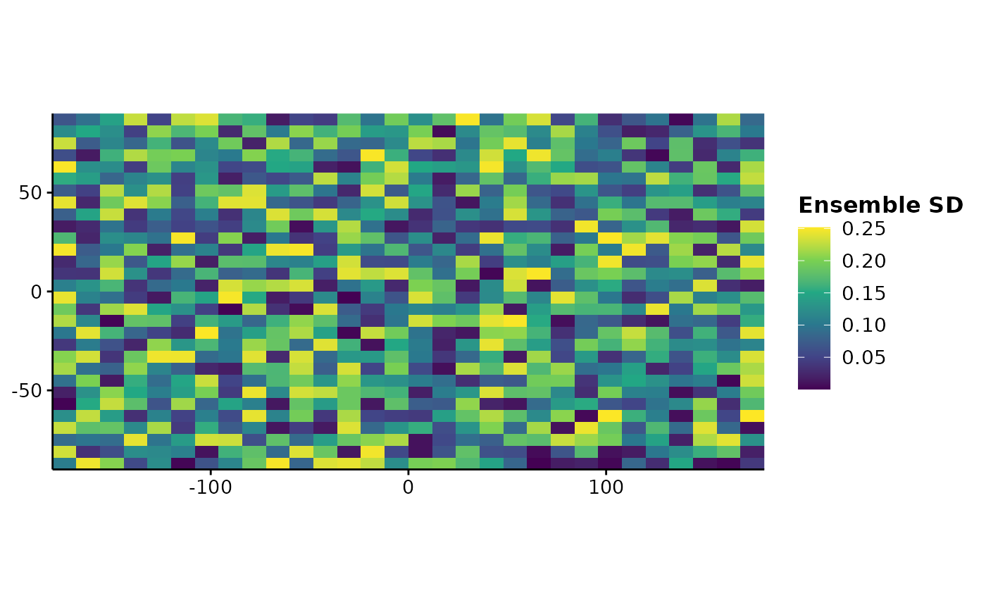
Draws the spread across an ensemble of projections. The companion to a projection map rather than a replacement for it: the two together say what the ensemble expects and where it is least sure.

Usage

plotUncertainty(
  x,
  statistic = c("sd", "cv", "range", "iqr"),
  na.rm = FALSE,
  title = "",
  legend.lab = NULL,
  max.cells = 5e+05,
  theme = theme_fancyfx(),
  option = "viridis"
)

Arguments

x

A SpatRaster whose layers are ensemble members, or a single-layer raster already summarised.

statistic

Spread statistic, passed to ensemble_summary(). Ignored when x has one layer.

na.rm

Whether to ignore missing members. Defaults to FALSE; see ensemble_summary().

title

Plot title, optional.

legend.lab

Legend title. Defaults to naming the statistic.

max.cells

Largest number of cells to draw. A raster above this is aggregated first, and the plot says by how much. See Details.

theme

A ggplot2 theme. Defaults to theme_fancyfx().

option

Viridis colour map option, passed to ggplot2::scale_fill_viridis_c().

Value

A ggplot2 object.

Details

Uncertainty is a magnitude, so it gets a sequential, perceptually uniform viridis scale rather than a rainbow – on a rainbow the eye invents boundaries where the data has none, which on an uncertainty map means inventing places the ensemble agreed.

Projection rasters are routinely millions of cells, and drawing one cell per pixel is both slow and pointless at figure size. Above max.cells the raster is aggregated by whole-number factors before plotting. That changes what is on the page, so it is reported in the subtitle rather than done quietly.

See also

ensemble_summary() for the raster itself, plotExtrapolation() for whether the projection is extrapolating.

Other spatial plots: ensemble_summary(), hex_bin(), mess(), niche_equivalency(), niche_overlap(), plot.fancyfx_equivalency(), plotExtrapolation(), plotHexbin(), thin_points()

Examples

if (requireNamespace("terra", quietly = TRUE)) {
  set.seed(1)
  r <- terra::rast(nrows = 30, ncols = 30, vals = runif(900))
  ensemble <- c(r, r * 1.2, r * 0.7)
  names(ensemble) <- c("model1", "model2", "model3")

  plotUncertainty(ensemble)
}