A surface and its uncertainty, as one figure
Usage
map_pair(
  x,
  value,
  uncertainty,
  uncertainty_from = NULL,
  by = NULL,
  coords = NULL,
  crs = NULL,
  kind = c("surface", "probability"),
  uncertainty_kind = c("surface", "diverging"),
  uncertainty_midpoint = 0,
  uncertainty_direction = 1,
  labels = NULL,
  titles = NULL,
  ncol = 2,
  coastline = TRUE,
  region = NULL,
  transform = "auto",
  limits = NULL,
  probs = c(0, 0.99),
  title = NULL,
  subtitle = NULL,
  caption = NULL,
  scalebar = TRUE,
  north = TRUE,
  scalebar_position = "bl",
  north_position = "tr",
  graticule = FALSE,
  base_size = 12,
  expand = 0.02
)
Arguments
- x
The geometry, or a
map_data. Both panels are drawn from it unlessuncertainty_fromnames a different object.- value
What the left panel colours by.
- uncertainty
What the right panel colours by: a CV, a standard error, a posterior standard deviation, an extrapolation score.
- uncertainty_from
A second object to take
uncertaintyfrom, when it does not live alongsidevalue. Must cover the same cells.- by, coords, crs
Passed to
as_map_data().crsis also the CRS the map is drawn in – seedisplay_crs()for what happens when it is not given.- kind
How the left panel is scaled:
"surface"for a skewed positive quantity,"probability"for one bounded at 0 and 1.- uncertainty_kind
How the right panel is scaled.
"surface"for a CV or an SE, which only increase;"diverging"for a signed score such as an extrapolation surface, which needsuncertainty_midpoint.- uncertainty_midpoint
The centre for a diverging right panel. Zero is the usual meaning and it is the default here, unlike in
map_diverging(), because the caller has already said the panel is diverging.- uncertainty_direction
Which way the diverging ramp runs on the right panel.
-1puts the warm arm at the low end, which is what an extrapolation surface wants.- labels
A length-2 character vector naming the two quantities in their legends.
- titles
A length-2 character vector of panel titles.
- ncol
Panels per row. Two side by side by default;
1stacks them, which suits a tall study area.- coastline
Where land comes from.
TRUEchooses a source for the extent,FALSEdraws none, a path or ansfobject supplies one. Seecoastline().- region
An
sfpolygon to outline over the map – the study area, or whatever the grid was cropped to.- transform, limits, probs
Passed to
surface_scale(), which decides how the values are ramped and says so.- title, subtitle, caption
Figure text. The caption is where provenance belongs: which period, which product, which correction was not applied. Anything this function had to decide – a capped scale, a missing coastline – is appended to it.
- scalebar, north
Whether to draw the furniture. See
scale_bar()andnorth_arrow().- scalebar_position, north_position
Which corner each sits in:
"bl","br","tl"or"tr". Two pieces of furniture asked into the same corner are warned about rather than moved – which corner is free depends on where the data sits, and only the caller can see that.- graticule
Whether to label coordinates. Off by default; see
theme_fancymap().- base_size
Base font size in points.
- expand
How much margin to leave around the data, as a fraction of its own extent. Widen it when the data does not reach anything a reader can orient by – a small grid in open water shows no coastline at all until the panel is wide enough to include one.
Details
Both panels are drawn on the same extent – the union of the two, so neither is cropped – in the same projection, with the same coastline object, and the furniture is drawn on the left panel only, since a scale bar repeated on an identical extent is furniture twice.
The two legends stay separate, and deliberately: they are different quantities in different units, and a shared one would be a lie. What they share is position, size and typography, which is what makes the pairing read.
Examples
grid <- example_grid()
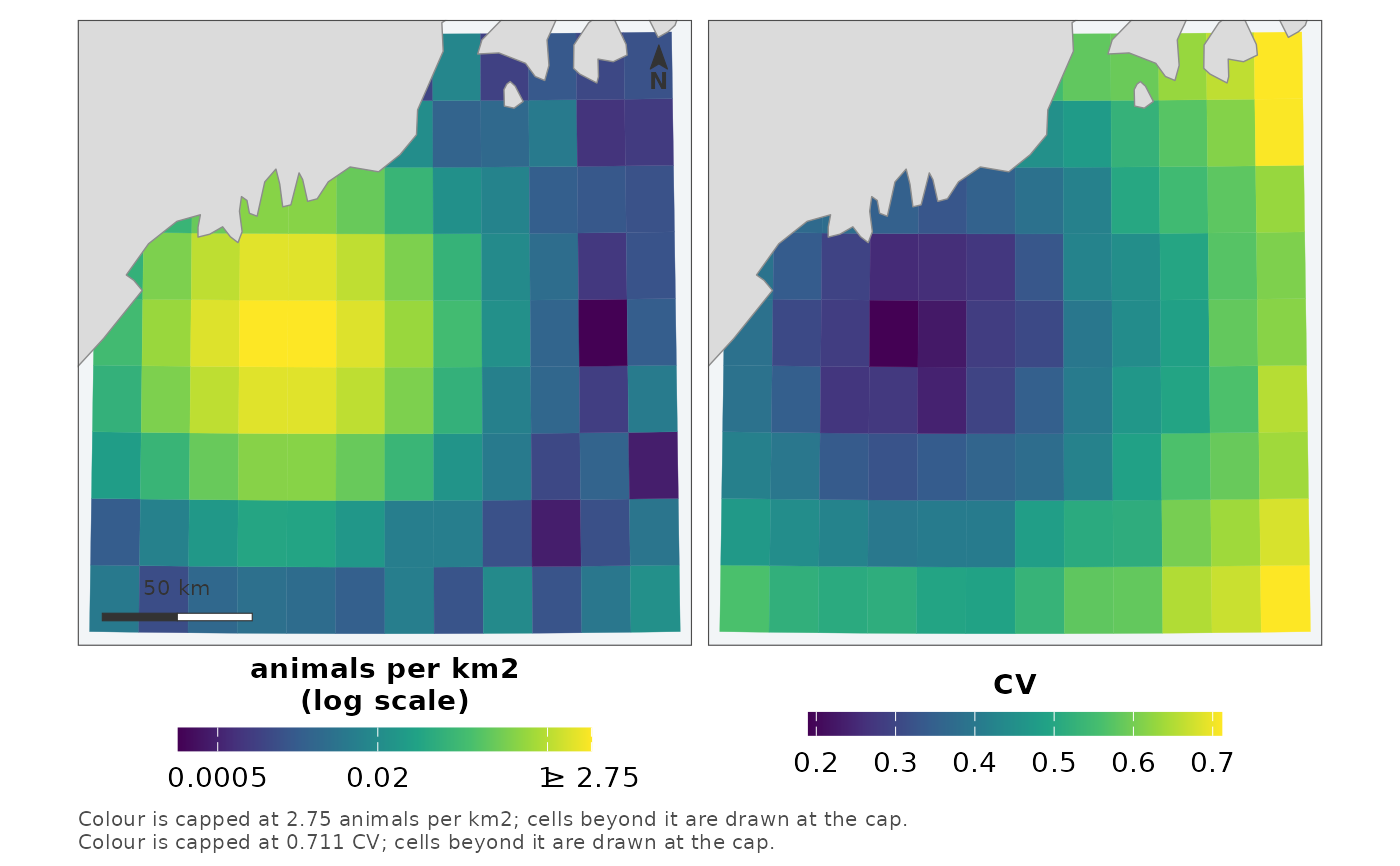
map_pair(grid, "density", "cv",
labels = c("animals per km2", "CV"))
#> scale: log, chosen because the 99th percentile is 170 times the median.
#> Pass `transform =` to fix it, if two figures need to match.
 # the projection-and-extrapolation pair
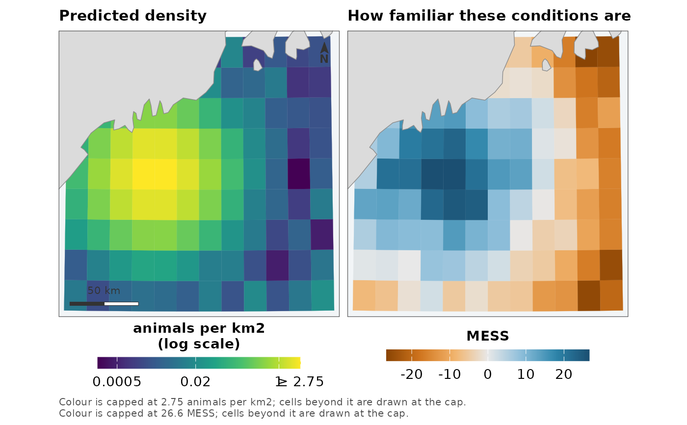
map_pair(grid, "density", "mess",
uncertainty_kind = "diverging", uncertainty_direction = -1,
labels = c("animals per km2", "MESS"),
titles = c("Predicted density",
"How familiar these conditions are"))
#> scale: log, chosen because the 99th percentile is 170 times the median.
#> Pass `transform =` to fix it, if two figures need to match.
# the projection-and-extrapolation pair
map_pair(grid, "density", "mess",
uncertainty_kind = "diverging", uncertainty_direction = -1,
labels = c("animals per km2", "MESS"),
titles = c("Predicted density",
"How familiar these conditions are"))
#> scale: log, chosen because the 99th percentile is 170 times the median.
#> Pass `transform =` to fix it, if two figures need to match.