Map a probability

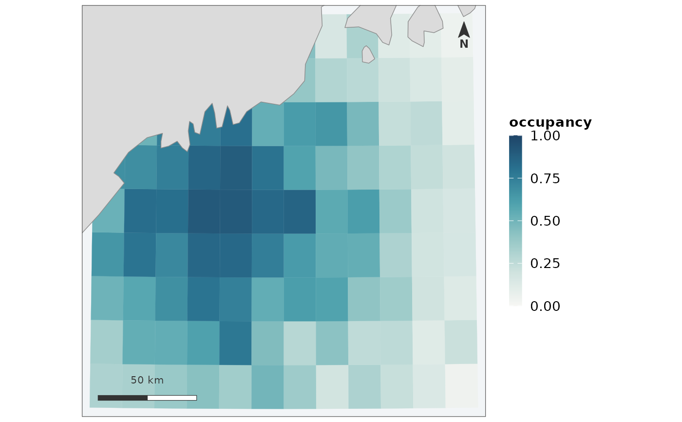
For a quantity that lives on [0, 1]: posterior occupancy, probability of presence, the proportion of ensemble members that agreed.

Usage

map_probability(
  x,
  value = NULL,
  by = NULL,
  coords = NULL,
  crs = NULL,
  label = NULL,
  coastline = TRUE,
  region = NULL,
  limits = c(0, 1),
  title = NULL,
  subtitle = NULL,
  caption = NULL,
  scalebar = TRUE,
  north = TRUE,
  scalebar_position = "bl",
  north_position = "tr",
  inset = FALSE,
  inset_position = "br",
  inset_size = 0.3,
  inset_zoom = 8,
  graticule = FALSE,
  base_size = 12,
  theme = NULL,
  expand = 0.02
)

Arguments

x

The geometry. An sf object of polygons, points or lines, a terra SpatRaster, or a data frame with coordinate columns. See as_map_data().

value

What to colour by: a column name, a vector in feature order, or a named vector joined by by. See as_map_data().

by, coords, crs

Passed to as_map_data(). crs is also the CRS the map is drawn in – see display_crs() for what happens when it is not given.

label

What to call the value in the legend. Defaults to the column name.

coastline

Where land comes from. TRUE chooses a source for the extent, FALSE draws none, a path or an sf object supplies one. See coastline().

region

An sf polygon to outline over the map – the study area, or whatever the grid was cropped to.

limits

The ends of the scale. c(0, 1) by default, and changing it is usually a mistake – see below.

title, subtitle, caption

Figure text. The caption is where provenance belongs: which period, which product, which correction was not applied. Anything this function had to decide – a capped scale, a missing coastline – is appended to it.

scalebar, north

Whether to draw the furniture. See scale_bar() and north_arrow().

scalebar_position, north_position

Which corner each sits in: "bl", "br", "tl" or "tr". Two pieces of furniture asked into the same corner are warned about rather than moved – which corner is free depends on where the data sits, and only the caller can see that.

inset

Whether to draw a locator inset – a small wider map with this figure's extent marked on it. FALSE by default, unlike the scale bar and north arrow, because an inset sits over a corner of the data rather than in a margin. TRUE uses the same coastline source as the map; a path or an sf object gives the inset its own.

inset_position, inset_size, inset_zoom

Which corner the inset sits in, how much of the panel width it takes, and how many times wider than the map it starts. See locator_inset() – inset_zoom is a starting point, not a setting, because an inset showing nothing but water orients nobody.

graticule

Whether to label coordinates. Off by default; see theme_fancymap().

base_size

Base font size in points.

theme

A theme to use instead of theme_fancymap().

expand

How much margin to leave around the data, as a fraction of its own extent. The default is a thin margin. Widen it when the data does not reach anything a reader can orient by – a small grid in open water shows no coastline at all until the panel is wide enough to include one.

Value

A ggplot2 object.

Details

A probability is not a skewed positive quantity with a coincidental upper bound, and drawing it with map_surface() gets two things wrong.

The scale is fixed at 0 and 1, not taken from the data. A map whose occupancy ran from 0.2 to 0.6 and was stretched across the full ramp says "high here, low there" in exactly the colours a map running 0 to 1 would use, and the two are not the same claim. Fixed ends also mean 0.6 is the same colour in every figure, which is what makes a series of years comparable at a glance.

The ramp is different. A sequential ramp puts its most saturated colour at the top of the data; here the top is certainty, and a cell at 0.02 should look nearly like a cell at 0, with weight arriving only as the value approaches 1.

Values outside [0, 1] are drawn at the ends and reported. A posterior mean cannot leave the interval, but a rescaled index or a ratio mistaken for a probability can, and that is worth being told about rather than clipping quietly.

See also

map_surface(), map_panels() for the same grid across seasons.

Examples

grid <- example_grid()
map_probability(grid, "occupancy", label = "occupancy")