The primary deliverable of a spatial model: a predicted quantity per cell, over a grid, with land, a stated projection and a scale that was chosen.
Usage
map_surface(
  x,
  value = NULL,
  by = NULL,
  coords = NULL,
  crs = NULL,
  label = NULL,
  coastline = TRUE,
  region = NULL,
  transform = "auto",
  limits = NULL,
  probs = c(0, 0.99),
  title = NULL,
  subtitle = NULL,
  caption = NULL,
  scalebar = TRUE,
  north = TRUE,
  scalebar_position = "bl",
  north_position = "tr",
  inset = FALSE,
  inset_position = "br",
  inset_size = 0.3,
  inset_zoom = 8,
  graticule = FALSE,
  base_size = 12,
  theme = NULL,
  expand = 0.02
)
Arguments
- x
The geometry. An
sfobject of polygons, points or lines, a terraSpatRaster, or a data frame with coordinate columns. Seeas_map_data().- value
What to colour by: a column name, a vector in feature order, or a named vector joined by
by. Seeas_map_data().- by, coords, crs
Passed to
as_map_data().crsis also the CRS the map is drawn in – seedisplay_crs()for what happens when it is not given.- label
What to call the value in the legend. Defaults to the column name.
- coastline
Where land comes from.
TRUEchooses a source for the extent,FALSEdraws none, a path or ansfobject supplies one. Seecoastline().- region
An
sfpolygon to outline over the map – the study area, or whatever the grid was cropped to.- transform, limits, probs
Passed to
surface_scale(), which decides how the values are ramped and says so.- title, subtitle, caption
Figure text. The caption is where provenance belongs: which period, which product, which correction was not applied. Anything this function had to decide – a capped scale, a missing coastline – is appended to it.
- scalebar, north
Whether to draw the furniture. See
scale_bar()andnorth_arrow().- scalebar_position, north_position
Which corner each sits in:
"bl","br","tl"or"tr". Two pieces of furniture asked into the same corner are warned about rather than moved – which corner is free depends on where the data sits, and only the caller can see that.- inset
Whether to draw a locator inset – a small wider map with this figure's extent marked on it.
FALSEby default, unlike the scale bar and north arrow, because an inset sits over a corner of the data rather than in a margin.TRUEuses the same coastline source as the map; a path or ansfobject gives the inset its own.- inset_position, inset_size, inset_zoom
Which corner the inset sits in, how much of the panel width it takes, and how many times wider than the map it starts. See
locator_inset()–inset_zoomis a starting point, not a setting, because an inset showing nothing but water orients nobody.- graticule
Whether to label coordinates. Off by default; see
theme_fancymap().- base_size
Base font size in points.
- theme
A theme to use instead of
theme_fancymap().- expand
How much margin to leave around the data, as a fraction of its own extent. The default is a thin margin. Widen it when the data does not reach anything a reader can orient by – a small grid in open water shows no coastline at all until the panel is wide enough to include one.
What it does not do
It does not compute the surface. Density, abundance, occupancy and their uncertainties are the fitting package's job; this draws what it is handed.
Skewed quantities
Predicted density is usually extremely skewed, and by default the scale
notices: see surface_scale() for the rule, which is reported whenever it
fires. For a probability, use map_probability(), whose scale is bounded at
0 and 1 rather than at whatever the data reached.
See also
map_probability() for a bounded quantity, map_diverging() for
one with a meaningful centre, map_pair() to draw one beside its
uncertainty.
Examples
grid <- example_grid()
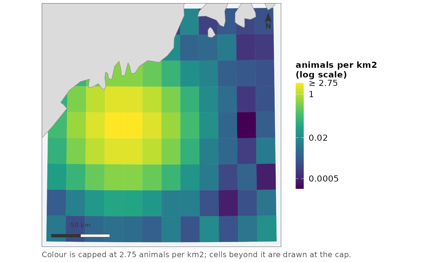
map_surface(grid, "density", label = "animals per km2")
#> scale: log, chosen because the 99th percentile is 170 times the median.
#> Pass `transform =` to fix it, if two figures need to match.
 # a fixed scale, for comparing with another figure
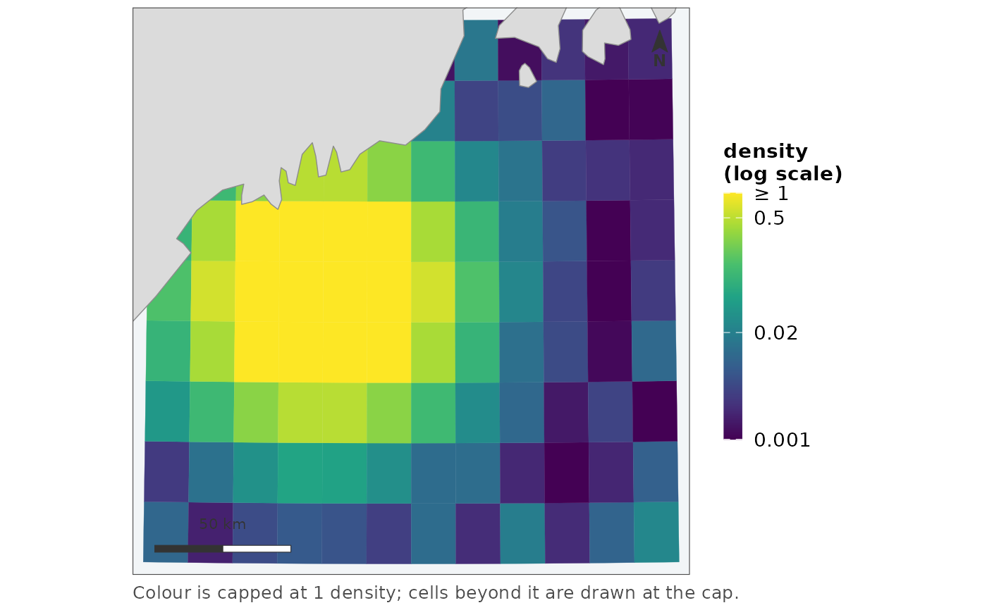
map_surface(grid, "density", transform = "log", limits = c(0.001, 1))
# a fixed scale, for comparing with another figure
map_surface(grid, "density", transform = "log", limits = c(0.001, 1))