Compare the same effect across several models

Plots one variable's effect from each of several models, side by side, so competing specifications can be read against each other. The companion to combinePlots(), which holds the model fixed and varies the predictor.

Usage

comparePlots(
  models,
  dat,
  var,
  title = "",
  xlab = NULL,
  ylab = NULL,
  transform = c("none", "log", "log10", "sqrt"),
  scale = c("auto", "link", "response"),
  interval = c("auto", "se", "ci", "cri"),
  level = 0.95,
  n = 100,
  rug.type = c("histogram", "density"),
  bins = 30,
  common.legend = TRUE,
  labels = "A",
  label.size = 14,
  title.size = 14,
  ...
)

Arguments

models: A list of fitted models. Names become the panel titles; if the list is unnamed, panels are titled "Model 1", "Model 2", and so on. Models need not be of the same class – a GAM can be compared against a GLM, subject to the caveat below.
dat: Raw data the models were fitted on, for the rugs. One data frame used for every panel, or a list with one per model.
var: Name of the predictor to plot. One name used for every model, or one per model, for comparing specifications that name a term differently.
title: Overall title for the figure, optional.
xlab: Label for the x-axis of every panel. Defaults to var.
ylab: Label for the y-axis of every panel. Defaults per panel to the quantity that panel actually computed.
transform: How to transform the variable before plotting. One value used for every panel, or one per model.
scale: "auto", "link", or "response", passed to plotEffects().
interval: "se" or "ci", passed to plotEffects().
level: Confidence level used when interval = "ci".
n: Number of points at which to evaluate each effect.
rug.type: Type of rug plot to draw above each effect.
bins: Number of bins for a histogram rug.
common.legend: Whether the panels share one legend. Worth turning off when the models are split by different factors, since a shared legend would then describe only the first.
labels: Panel labels: "A" (the default) for upper-case letters, "a" for lower-case, "1" for numbers, "none" for none, or a character vector used verbatim, one per panel.
label.size: Font size of the panel labels. These are drawn by the arranging step rather than by the theme, so they do not follow base_size and have to be set here.
title.size: Font size of the overall figure title, for the same reason.
...: Passed through to plotEffects() and on to the backend.

Value

The arranged plots, as returned by ggpubr::ggarrange().

Details

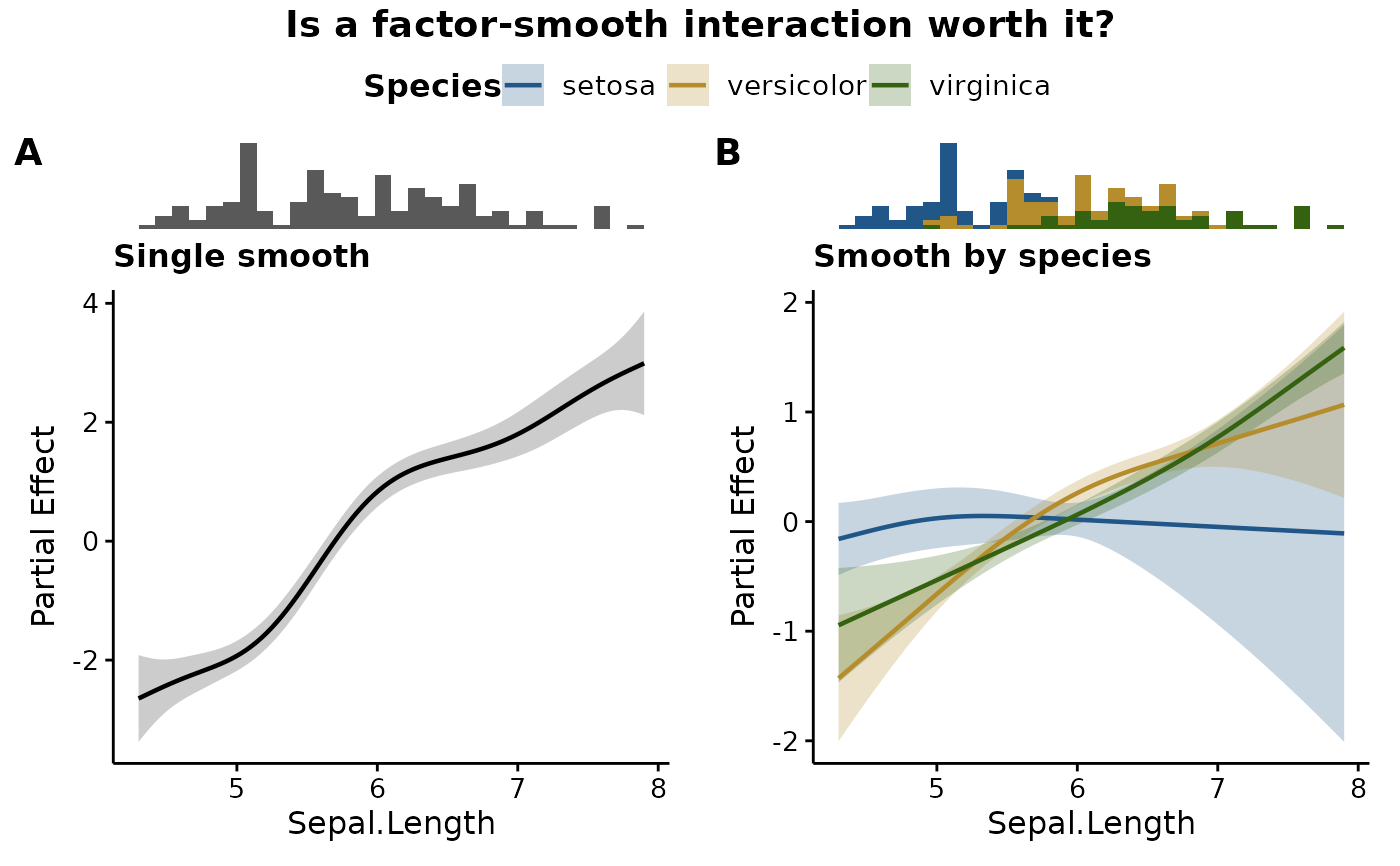
The motivating case is asking what a modelling choice actually bought you: fit the same data with and without a factor-smooth interaction, put the two panels next to each other, and see whether the smooths really do differ by group. Each panel keeps its own rug, so a group with little data is visible rather than inferred.

Comparing like with like

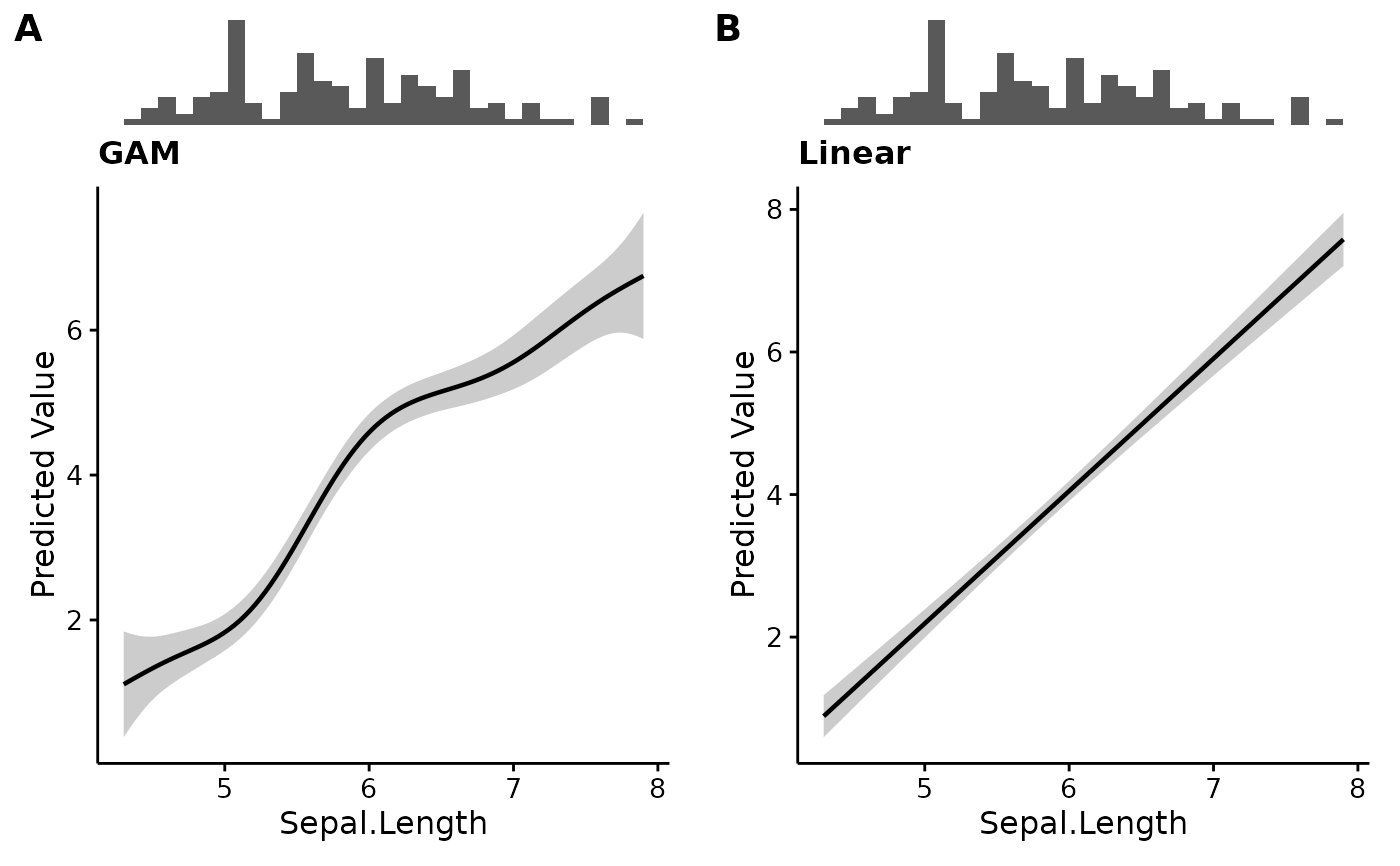
Panels are only comparable if they show the same quantity. A GAM defaults to its partial effect and a GLM to its predictions, and putting those side by side compares a curve centered on zero against one that is not. When the models are of different classes, pass scale = "response" so every panel reports predictions, or read the y-axis labels carefully – they will differ, which is the signal that the panels are not on the same footing.

Examples

# Does letting the smooth vary by species actually buy anything?
plain <- mgcv::gam(Petal.Length ~ s(Sepal.Length), data = iris)
by.species <- mgcv::gam(Petal.Length ~ s(Sepal.Length, by = Species) + Species,
                        data = iris)

comparePlots(list("Single smooth" = plain,
                  "Smooth by species" = by.species),
             iris, "Sepal.Length",
             title = "Is a factor-smooth interaction worth it?")


# Comparing across model classes: ask for the same quantity from both.
comparePlots(list(GAM = plain, Linear = lm(Petal.Length ~ Sepal.Length, iris)),
             iris, "Sepal.Length", scale = "response")