Research
Estimating ecological fields from sparse, irregular, effort-limited observations — and keeping the observation process separate from the ecological one.
Our knowledge of whales at sea is contingent upon our ability to find them: whether visually from an airplane or vessel or acoustically from hydrophones. Both of those observation types are shaped as much by the survey as by the animal’s behavior and environmental conditions.
My work as a biological oceanographer focused on conservation considers what we can infer from the data we are able to collect. I build models that separate the observation process from the ecological process, so that what comes out the other end is an estimate of what is actually there rather than an estimate of where we happened to look. That matters because these models are not academic exercises: they are considered by the entities who build the tools used to manage the critically endangered North Atlantic right whale.
Whale prey
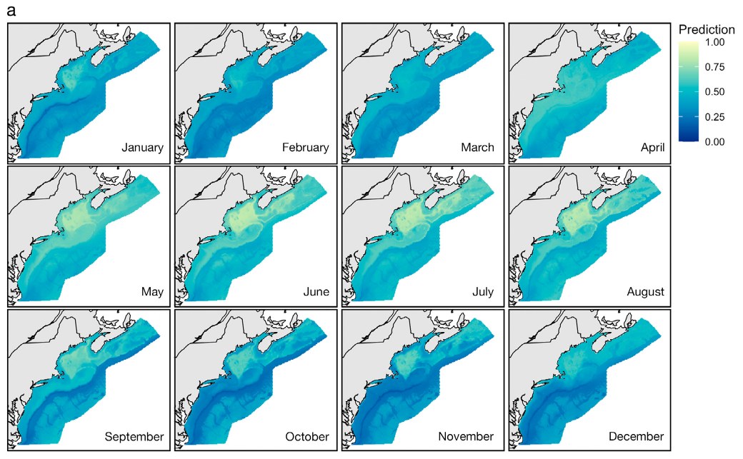
Right whales eat copepods — primarily Calanus finmarchicus. However, a whale does not necessarily respond to average copepod abundance, but rather to whether a prey patch is dense enough that feeding on it is energetically advantageous. That distinction matters especially for modeling.
Part of my work involves using environmental conditions to explain and predict prey aggregations that exceed a whale-specific feeding threshold. We refer to these high-density prey aggregations as τ-patches. This modeling strategy differs from abundance-based models: we are able to interpolate zooplankton data in a given region, like the Gulf of Maine, from the perspective of a foraging whale. This led to new prey covariate fields that have proven useful in right whale density surface models. The approach has been extended beyond C. finmarchicus to Centropages typicus and Pseudocalanus spp., revealing that the τ-patch probability shifts not only between species, but across space and time.
Key papers: Estimating right whale prey based on Calanus finmarchicus thresholds · Beyond Calanus: changes to the copepod community · Calanus species and foraging habitat in Canadian waters
Code: taupatch implements
the threshold patch models;
datamatch and
derivoce build the
environmental covariates.
Whale habitat preference
Density surface models turn systematic line-transect survey data into maps of animal density. They are only as good as their treatment of the observation process: how detectability falls off with distance, how effort is distributed, how much of the variance in a map is survey design rather than biology.
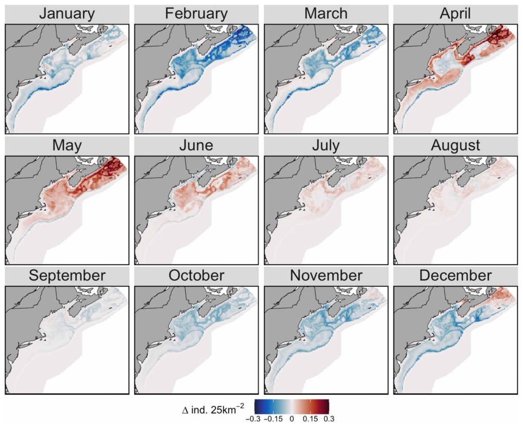
A central theme of my work has been designing prey covariates and testing how they can improve endangered species habitat models. Marine habitat models conventionally rely upon chlorophyll-a concentration or NPP models as a proxy for zooplankton prey. However, satellite- or model-derived chlorophyll products are several steps removed from the food right whales are actually targeting. We have found that substituting whale-specific prey fields for prey proxies improves right whale density model distributions: in a recent paper, combining three right whale-specific copepod prey fields improved density estimates to closer represent what we would expect in the field.
This work emphasizes the need for continued surveying and sampling of both whales and zooplankton.
Key papers: Incorporating prey fields into right whale density surface models · Impacts of an oceanographic regime shift on U.S. right whale density estimates (in review)
Code: narwcr and
distsamp handle survey ingest
and segmentation; dsfit fits and
compares detection functions on effective strip half-width rather than
the Akaike information criterion (AIC) alone.
Looking to the future
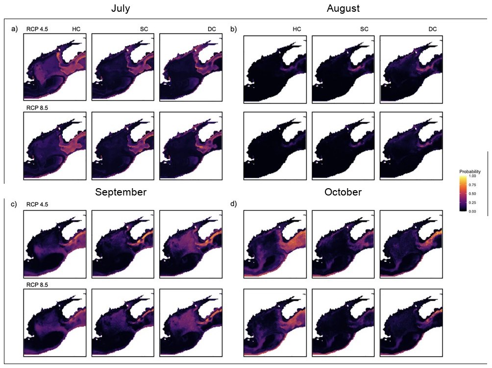
The Gulf of Maine is warming faster than the rest of the ocean, and right whales have already redistributed in ways that broke the assumptions behind existing management strategies and surveying designs. Projecting habitat suitability forward into 2050 under different IPCC climate scenarios suggests the trend continues: declining suitability across much of the Gulf of Maine from mid-summer into autumn, with a north-eastward shift toward the Scotian Shelf, the Bay of Fundy, and the Newfoundland and Labrador shelves — much of it outside where conservation effort has been historically concentrated.
Change of this scale presents on decadal as well as on interannual and monthly scales. The Gulf of Maine has a documented history of unprecedented oceanographic conditions, arriving with increasing frequency than the decadal-scale trends alone would predict. That raises a harder question than “what will the mean look like in 2050”: what happens to a density estimate built across distinct oceanographic regimes, when the relationship the model learned no longer holds? This is the underlying question of much of my current work.
Key papers: Projecting right whale habitat suitability for 2050 · Foraging habitat under future climate scenarios · The surprising oceanography of the Gulf of Maine
Methods and tools
- Observation process — detectability modeling from line-transect data, density surface models with explicit treatment of survey effort, propagating observation uncertainty into management-facing estimates
- Statistical learning — generalized additive models, boosted regression trees, random forests, artificial neural networks (including CNNs trained from scratch)
- Time series — spectral analysis of multi-decadal oceanographic and biological series: Fourier transforms and periodograms, coherence, filtering, autocorrelation structure
- Data sources — Copernicus Earth Observation and NASA EarthData products, ocean physics model output (HYCOM, GLORYS, FVCOM, DFO internal models), aerial and vessel survey archives, passive acoustic monitoring
- Practice — R, Python, git, bash, Linux; reproducible pipelines; R Shiny and Leaflet
Background reading
Foundational works for this research, including modeling methods and the current state of the ecosystem.
- Mayo, C. A., Marx, M. K. (1990). Surface foraging behaviour of the North Atlantic right whale, Eubalaena glacialis, and associated zooplankton characteristics. Canadian Journal of Zoology.The foundational description of how these whales actually feed.
- Miller, D. L., Burt, M. L., Rexstad, E. A., Thomas, L. (2013). Spatial models for distance sampling data: recent developments and future directions. Methods in Ecology and Evolution.The density surface modeling framework this work builds on.
- Pershing, A. J., Alexander, M. A., Hernandez, C. M., Kerr, L. A., et al. (2015). Slow adaptation in the face of rapid warming leads to collapse of the Gulf of Maine cod fishery. Science.The warming that reshaped this ecosystem, and what it cost.
- Roberts, J. J., Best, B. D., Mannocci, L., Fujioka, E., Halpin, P. N., et al. (2016). Habitat-based cetacean density models for the U.S. Atlantic and Gulf of Mexico. Scientific Reports.The density models these prey fields are designed to feed into.
- Baumgartner, M. F., Wenzel, F. W., Lysiak, N. S. J., Patrician, M. R. (2017). North Atlantic right whale foraging ecology and its role in human-caused mortality. Marine Ecology Progress Series.Links where the whales feed to where they are killed.
- Record, N. R., Runge, J. A., Pendleton, D. E., Balch, W. M., et al. (2019). Rapid climate-driven circulation changes threaten conservation of endangered North Atlantic right whales. Oceanography.How circulation change moved the prey, and the whales with it.
- Sorochan, K. A., Plourde, S., Baumgartner, M. F., Johnson, C. L. (2021). Availability, supply, and aggregation of prey (Calanus spp.) in foraging areas of the North Atlantic right whale. ICES Journal of Marine Science.Why aggregation, not abundance, is the quantity that matters.
- Pershing, A. J., Alexander, M. A., Brady, D. C., Brickman, D., et al. (2021). Climate impacts on the Gulf of Maine ecosystem. Elementa: Science of the Anthropocene.A synthesis of how the Gulf of Maine is changing.
- Meyer-Gutbrod, E. L., Greene, C. H., Davies, K. T. A., Johns, D. G. (2021). Ocean regime shift is driving collapse of the North Atlantic right whale population. Oceanography.The regime shift framing, applied to this population.