Bin point values into a hexagonal surface

Points with a value each in, one sf polygon per occupied hexagon out, with the values summarised per bin. The binned form of a quantity, ready to hand to whichever map verb suits it.

Usage

hex_surface(
  x,
  value = NULL,
  bins = 30,
  fun = "mean",
  coords = NULL,
  crs = NULL
)

Arguments

x

Points: an sf object, or a data frame with coordinate columns.

value

The value to summarise: a column name or a vector, as in as_map_data(). NULL counts points instead.

bins, fun

How many hexagons across the extent, and how the values in each are summarised – any fun fancyfx::hex_bin() takes.

coords, crs

As in as_map_data().

Value

An sf data frame with one row per occupied hexagon: value, the summarised quantity; n, how many points fell in the bin; and the hexagon's polygon.

Details

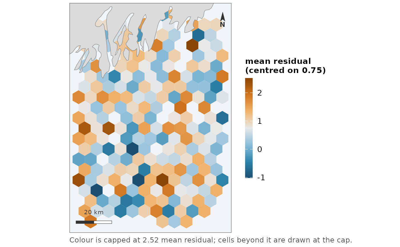
map_effort() bins for you, and always onto a sequential scale, which is right for the question it asks – how much, where. This is the way out when the binned quantity needs a different scale. The first customer is model residuals: binned because 8,000 overlapping segments cannot show a cluster, and then diverging, centred on the survey's own mean residual, because deviance residuals do not average zero:

hex <- hex_surface(segments, "resid", fun = "mean")
map_diverging(hex, "value", midpoint = mean(hex$value))

Binning happens in the display projection, not in lon/lat, for the reason map_effort()'s binning does: hexagons binned in degrees are not hexagons on a map, by the same factor that makes a degree of longitude 74 km in the Gulf of Maine and 111 at the equator.

See also

map_effort() for the count-where-the-effort-was case, map_diverging() for drawing the result on a centred scale.

Examples

pts <- sf::st_as_sf(
  data.frame(lon = runif(500, -70, -69), lat = runif(500, 43, 44),
             resid = rnorm(500, mean = 0.8)),
  coords = c("lon", "lat"), crs = 4326)

hex <- hex_surface(pts, "resid", bins = 12, fun = "mean")
map_diverging(hex, "value", midpoint = mean(hex$value),
              label = "mean residual")