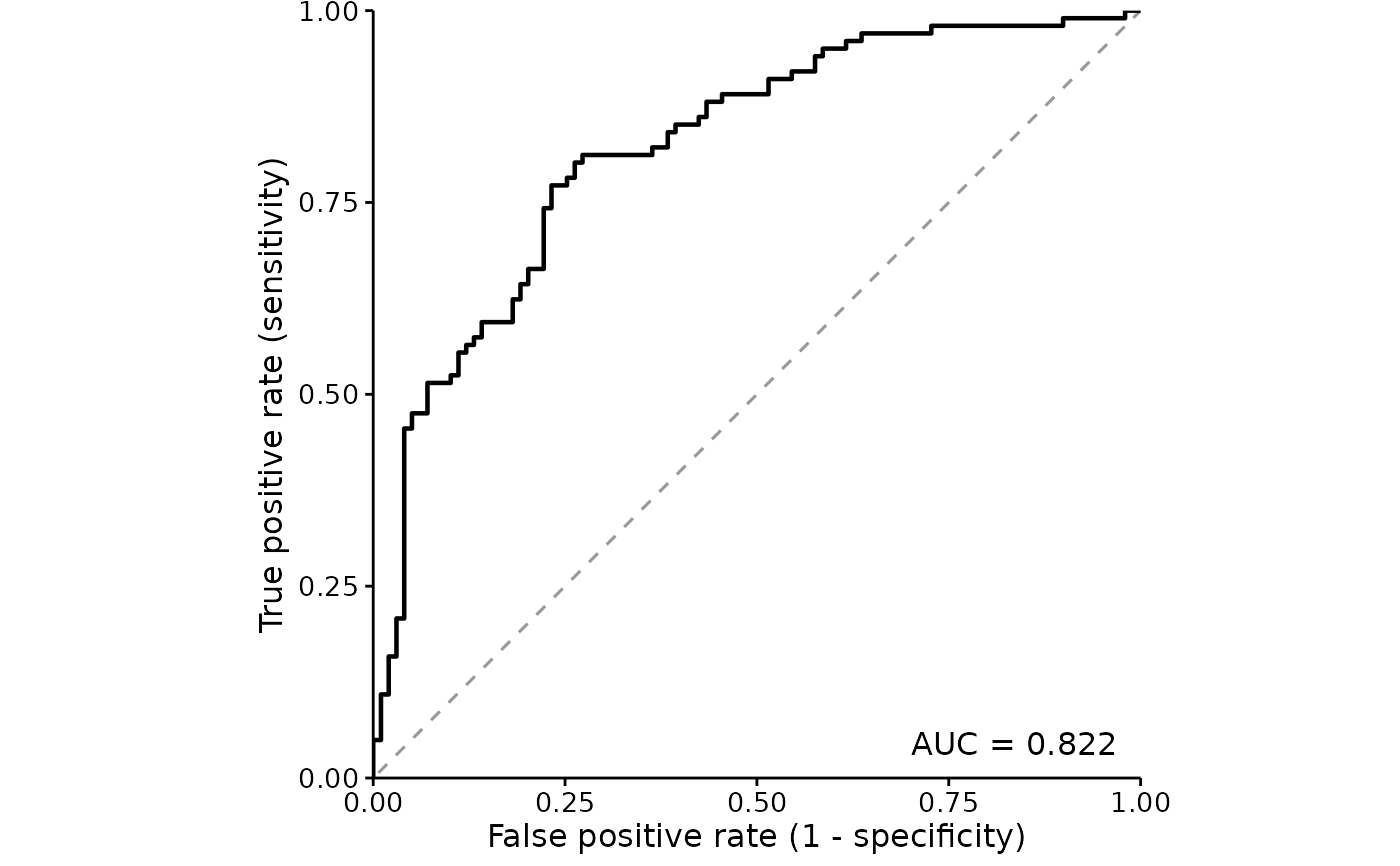
Sensitivity against the false positive rate across every cutoff, with the area under the curve reported. The diagonal is the reference: a model that ranks presences no better than chance lies on it.
Usage
plotROC(
  model,
  newdata = NULL,
  folds = NULL,
  title = "",
  show.auc = TRUE,
  theme = theme_fancyfx(),
  palette = fancyfx_palette(),
  linewidth = 0.8,
  ...
)
Arguments
- model
A fitted presence/absence model.
- newdata
Data to evaluate on. Required, and it should not be the data the model was fitted to – see
threshold_metrics().- folds
Optional fold identifiers, one per row of
newdata. Each fold is drawn as its own curve, so the spread is visible rather than averaged.- title
Plot title, optional.
- show.auc
Whether to report the AUC on the plot.
- theme
A ggplot2 theme. Defaults to
theme_fancyfx().- palette
Colours used for fold curves. Defaults to
fancyfx_palette().- linewidth
Width of the curve.
- ...
Passed to
threshold_metrics()and on tostats::predict().
Details
The plot is square with equal axes, because a ROC curve read on unequal axes misleads about how far from the diagonal it sits.
AUC is computed from ranks, not by integrating the drawn curve, so tied
predictions are handled exactly. With folds, one AUC per fold is reported
as a range rather than a mean: the spread is the informative part.
If the metrics came from the model's own training data, the plot says so beneath the axis. That annotation is not decoration – an in-sample ROC can look excellent for a model with no predictive value at all.
References
Allouche, O., Tsoar, A., & Kadmon, R. (2006). Assessing the accuracy of species distribution models: prevalence, kappa and the true skill statistic (TSS). Journal of Applied Ecology, 43(6), 1223-1232. doi:10.1111/j.1365-2664.2006.01214.x
See also
plotThreshold() for choosing a cutoff, threshold_metrics() for
the numbers underneath.
Other evaluation plots:
calc_deviance(),
calibration_estimates(),
held_out(),
permutation_importance(),
plotCalibration(),
plotImportance(),
plotThreshold(),
spatial_sorting_bias(),
threshold_metrics()